This server predicted 8 kinds of commonly used basic chemical properties. To predicted these properties, we search for as many as data sources from the public databases and scientific papers. Finally, we collected the 8 datasets and then employed several advanced QSAR methodologies to estimate these properties.
The density is defined as the mass per unit volume. The data set for this endpoint was obtained from the density data contained in LookChem (Lookchem.com 2011). The data set was restricted to chemicals with boiling points greater than 25°C (or the boiling point was unavailable). The data set was further restricted to chemical with densities greater than 0.5 and less than 5 g/cm3. The final dataset consisted of 8909 chemicals. The data in lookchem.com is not peer reviewed but the set is very large and thus provides a large degree of structural diversity. The modeled property was the density in g/cm3.
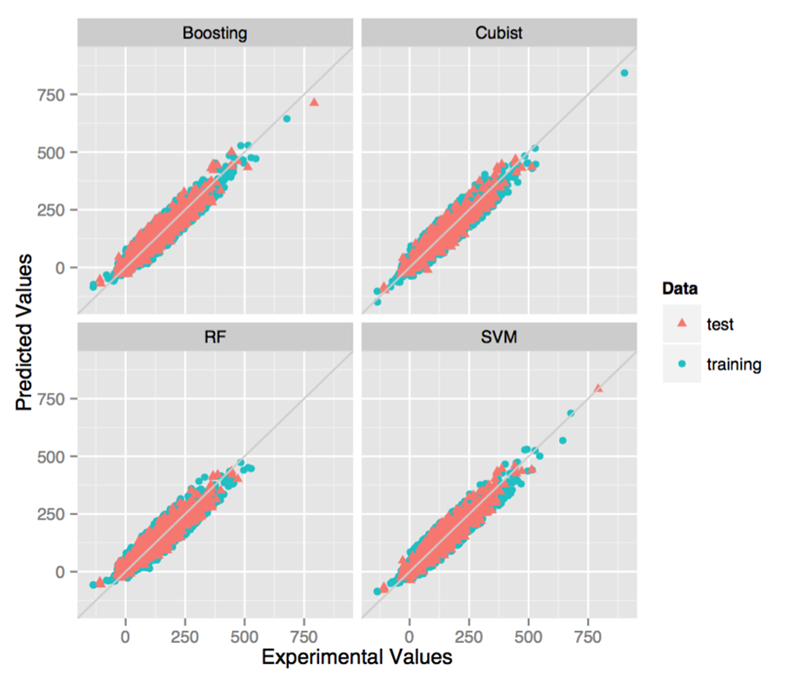
The flash point is defined as the lowest temperature at which a chemical can vaporize to form an ignitable mixture in air. A dataset of 8362 chemicals was also compiled from lookchem.com (Lookchem.com 2011). Chemicals with flash points greater than 1000°C were omitted from the data set. The modeled property was the flash point in °C.
Viscosity is a measure of the resistance of a fluid to flow in cP defined as the proportionality constant between shear rate and shear stress). The viscosity at 25°C for 557 chemicals was obtained from the data compilations of Viswanath and Riddick (Viswanath 1989; Riddick et al. 1986).
Surface tension is a property of the surface of a liquid that allows it to resist an external force. The surface tension at 25°C for 1416 chemicals was obtained from the data compilation of Jaspar (Jasper 1972). The experimental values (at 25°C) are estimated using an empirical correlation which is fit to experimental data from Jaspar: surface tension = A - BT. The estimated experimental surface tension value is only used if the closest experimental data point is within 10°C of 25°C. The modeled property was the surface tension in dyn/cm.
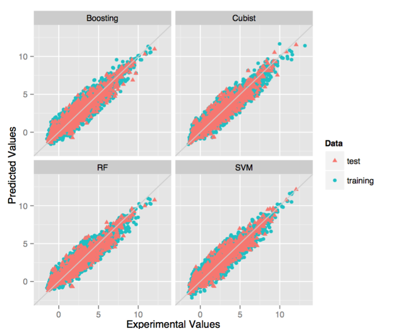
Vapor pressure is defined as the pressure of a vapor in mmHg in thermodynamic equilibrium with its condensed phases in a closed system. The vapor pressure at 25°C for 2511 chemicals was obtained from the database in EPI Suite (USEPA 2009). The modeled property was Log10(vapor pressure mmHg).
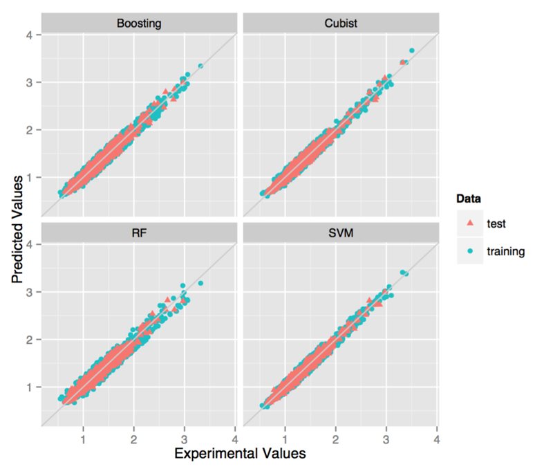
Melting point (the temperature in °C at which a chemical in the solid state changes to a liquid state). The melting point for 9385 chemicals was obtained from the database in EPI Suite (USEPA 2009). The modeled property was Log10(vapor pressure mmHg).
Water solubility is defined as the amount of a chemical in that will dissolve in liquid water to form a homogeneous solution. A dataset of 5020 chemicals was compiled from the database in EPI Suite (USEPA 2009). Chemicals with water solubilities exceeding 1,000,000 mg/L were omitted from the overall dataset. In addition the data was limited to data points that are within 10°C of 25°C. The water solubility is an important property because sometimes the predicted LC50 values for aquatic species can exceed the water solubility. The modeled property was -Log10(water solubility mol/L).
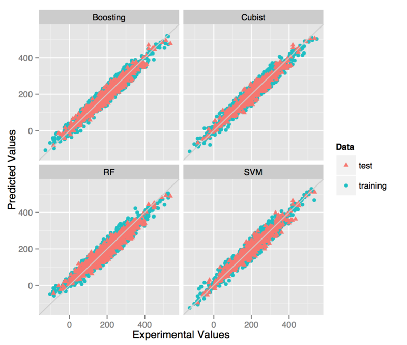
The normal boiling point is defined as the temperature at which a chemical boils at atmospheric pressure. The data set for this endpoint was obtained from the boiling point data contained in EPI Suite (USEPA 2009). 41 chemicals were removed from the data set since they were previously shown to be badly predicted and had experimental values which were significantly different (>50K) from other sources such as NIST(NIST 2010) and LookChem (Lookchem.com 2011). The final data set contained 5759 chemicals. The modeled property was the boiling point in °C.
Molecular polar surface area (PSA), i.e., surface belonging to polar atoms, is a descriptor that was shown to correlate well with passive molecular transport through membranes and, therefore, allows prediction of transport properties of drugs. Topology molecular surface area (TPSA) is a new approach for the calculation of the PSA for its fast calculation (J. Med. Chem., 2000, 43 (20), pp 3714–3717). MR is short for the Wildman-Crippen Molar refractivity value, and Log P represents partition coefficient of molecules (J. Chem. Inf. Comput. Sci., 1999, 39 (5), pp 868–873). These three properties were calculated by using RDKit packages.
To represent these molecules, we calculated 378 2D molecular descriptors from 11 feature groups using online molecular calculation platforms: ChemDes (http://www.scbdd.com/chemdes) and BioTriangle (http://biotriangle.scbdd.com). By using ChemDes and BioTriangle, the calculated values can be downloaded as a well-organized *.csv file, which could be used directly as inputs for the next modelling step. The 359 descriptors are: 30 constitutional descriptors, 44 connectivity descriptors, 35 topology descriptors, 7 Kappa descriptors, 32 Moran autocorrelation descriptors, 60 MOE-type descriptors, 21 Basak descriptors, 64 Burden descriptors, 6 Molecular property descriptors, 25 Charge descriptors and 89 E-state descriptors.
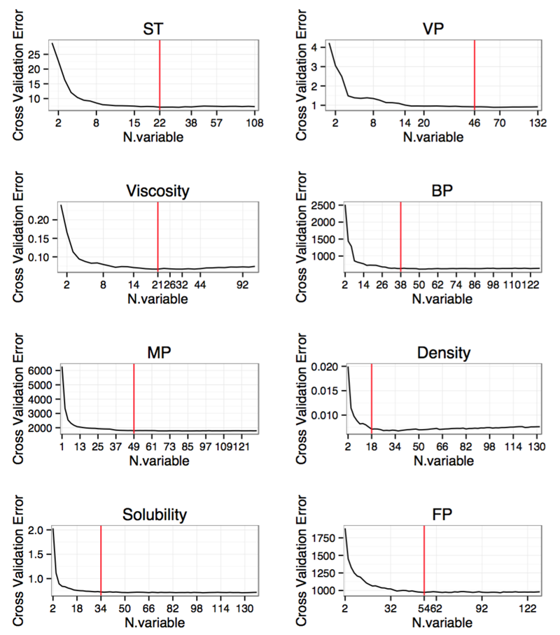
To improve accuracy scores of the QSAR models and to boost their performance on the datasets with quite many features, the feature selection process is needed. Here, we employed the randomForest algorithm to take a recursive feature elimination. According to the feature importance, we finally selected the features as follows: BP(short for 'Normal boiling point'): 38, density: 18, MP(short for 'Melting point'): 49, Solubility: 34, ST(short for 'Surface tension'): 22, Viscosity: 21, VP(short for 'Vapor pressure'): 46, FP(short for 'Flash point '): 54. The detailed information is shown as Table 1 and Figure 1.
| Data | Descriptor |
|---|---|
| BP | PC6, GMTIV, W, Chi8, Sitov, Gravto, Chiv8, TPSA, Save, ncarb, UI, Scar, IC6, Hy, slogPVSA9, bcutp10, dchi4, Smax, IC1, MRVSA9, KierA1, Tnc, Smin, S17, AWeight, bcutp15, bcutv12, ndonr, dchi0, Soxy, bcutv11, IVDE, Chiv2, LogP, Hatov, LogP2, dchi1, slogPVSA11 |
| Density | AWeight, MRVSA9, slogPVSA11, Hatov, Shet, Gravto, nhyd, Scar, S7, BertzCT, IC1, dchi0, CIC1, Save, TPSA, Smin, noxy, dchi4 |
| MP | TPSA, IC1, ndonr, noxy, GMTIV, dchi4, Tnc, UI, Gravto, Chi10, knotp, IVDE, Chi3c, Shet, dchi0, J, KierA3, W, bcutp2, dchi1, IC6, Kier3, CIC1, PEOEVSA0, nhet, Chiv4pc, IC2, bcutp3, knotpv, MRVSA9, Snitro, Hatov, naro, S36, Chiv10, nhyd, LogP, Save, Scar, Smin, S34, slogPVSA1, slogPVSA0, naccr, Hy, nring, CIC4, LogP2, Chiv3c |
| Solubility | LogP, LogP2, Tsch, Gravto, TPSA, Chiv8, bcutp2, Chi10, slogPVSA1, PEOEVSA5, MRVSA9, dchi4, Hy, GMTIV, UI, naccr, naro, bcutp3, Scar, Smax, Tpc, Smin, dchi1, AWeight, Shal, nhyd, knotp, dchi0, IC1, Save, PEOEVSA0, MZM1, CIC0, Hatov |
| ST | S7, UI, Hatov, dchi0, TPSA, IC1, BertzCT, AWeight, nhet, S12, MRVSA9, Gravto, Smax, S17, dchi3, dchi2, slogPVSA1, GMTIV, Smin, J, Save, nring |
| Viscosity | S34, PEOEVSA0, Tac, GMTIV, ndonr, Gravto, Chiv6, PC6, TPSA, Scar, bcutp3, Shev, Chiv2, BertzCT, LogP, bcutv10, DS, IVDE, slogPVSA1, Qindex, LogP2 |
| VP | GMTIV, W, Chi10, PC6, Chiv10, Shev, Gravto, Chiv6, TPSA, Tpc, IVDE, IC1, bcutp10, ncarb, Shet, ndonr, Save, nring, MZM2, J, PEOEVSA0, nhet, S38, MZM1, LogP, Hy, LogP2, CIC6, dchi0, Scar, dchi1, bcutv11, Smin, Hatov, AWeight, Shal, MRVSA0, Smax, Chi3c, slogPVSA9, S34, bcutp16, IC2, slogPVSA2, nsb, S35 |
| FP | GMTIV, TPSA, W, Chi10, Gravto, Tnc, Chiv10, IVDE, UI, dchi4, Shet, bcutp2, IC1, ndonr, dchi0, LogP, MRVSA9, Save, noxy, dchi2, IC5, naro, J, PEOEVSA0, Smax, Chiv2, Scar, LogP2, naccr, Snitro, Smin, bcutv11, Hy, AWeight, MZM2, Hatov, Chi3c, nnitro, S17, S36, slogPVSA1, MZM1, CIC6, S7, S34, S12, CIC1, knotp, Chiv4pc, slogPVSA9, KierA3, S35, IC2, nhyd |
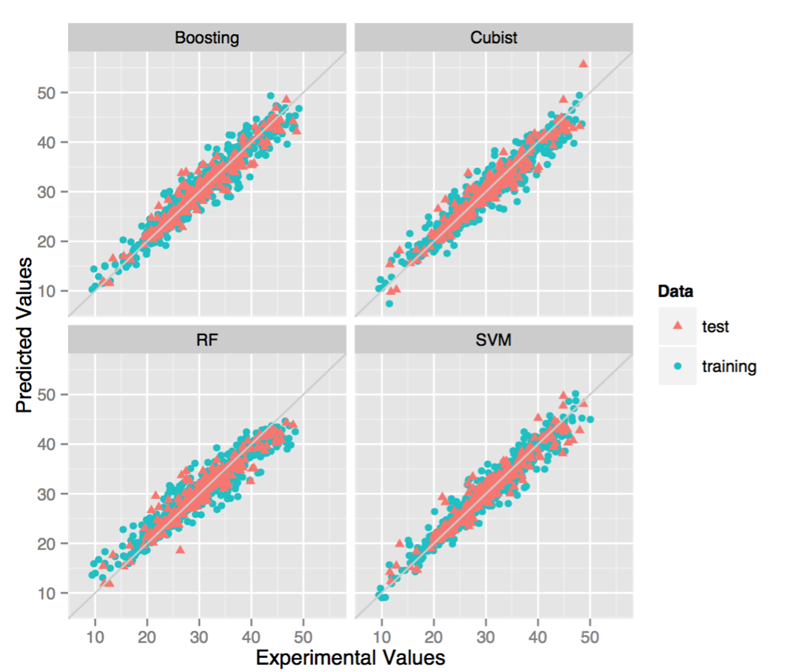
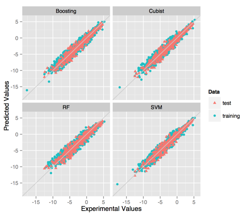
After the feature selection, we used the four state-of-arts machine learning algorithms to build models. In this step, we used the grid search method to optimize a best set of parameters for each model. The detailed information is shown in Table 2. As there may be several outliers which possess relatively large error, it is necessary to remove part of the molecule to improve the prediction accuracy. Here, we also tried to build models using datasets removing samples with prediction error greater than three times of RMSE.
| Data | Sample | Descriptors | Parameters | ||||
|---|---|---|---|---|---|---|---|
| Training/test | SVM | Boosting | |||||
| sigma | C | epsilon | shrinkage | depth | |||
| ST | 1133/283 | 22 | -7 | 6 | -4 | 0.06 | 8 |
| VP | 2006/504 | 46 | -7 | 3 | -8 | 0.06 | 8 |
| Viscosity | 444/113 | 21 | -5 | 5 | -3 | 0.01 | 6 |
| BP | 4607/1151 | 38 | -8 | 6 | -12 | 0.07 | 8 |
| Density | 7125/1783 | 18 | -7 | 6 | -8 | 0.05 | 7 |
| MP | 7509/1875 | 49 | -6 | 3 | -2 | 0.07 | 8 |
| Solubility | 4016/1004 | 34 | -6 | 4 | -3 | 0.06 | 8 |
| FP | 6690/1672 | 54 | -10 | 6 | -3 | 0.09 | 8 |
| Data | Methods | R2 | RMSEFit | Q2 | RMSECV | RT2 | RMSET |
|---|---|---|---|---|---|---|---|
| ST | Cubist | 0.951 | 1.45 | 0.868 | 2.38 | 0.908 | 2.07 |
| RF | 0.972 | 1.11 | 0.837 | 2.65 | 0.88 | 2.36 | |
| SVM | 0.946 | 1.53 | 0.895 | 2.12 | 0.868 | 2.48 | |
| Boosting | 0.992 | 0.589 | 0.863 | 2.43 | 0.912 | 2.03 | |
| VP | Cubist | 0.975 | 0.546 | 0.938 | 0.855 | 0.947 | 0.814 |
| RF | 0.987 | 0.39 | 0.922 | 0.959 | 0.931 | 0.933 | |
| SVM | 0.974 | 0.559 | 0.945 | 0.809 | 0.941 | 0.862 | |
| Boosting | 0.995 | 0.239 | 0.938 | 0.855 | 0.943 | 0.845 | |
| Viscosity | Cubist | 0.916 | 0.166 | 0.683 | 0.322 | 0.832 | 0.231 |
| RF | 0.962 | 0.112 | 0.8 | 0.256 | 0.805 | 0.248 | |
| SVM | 0.963 | 0.111 | 0.881 | 0.198 | 0.846 | 0.22 | |
| Boosting | 0.93 | 0.151 | 0.79 | 0.262 | 0.789 | 0.258 | |
| BP | Cubist | 0.973 | 13.9 | 0.942 | 20.4 | 0.94 | 20.9 |
| RF | 0.986 | 10.2 | 0.914 | 24.8 | 0.917 | 24.5 | |
| SVM | 0.955 | 18.1 | 0.936 | 21.5 | 0.929 | 22.7 | |
| Boosting | 0.988 | 9.31 | 0.94 | 20.8 | 0.934 | 21.9 | |
| Density | Cubist | 0.966 | 0.0601 | 0.955 | 0.0696 | 0.963 | 0.0614 |
| RF | 0.988 | 0.0363 | 0.933 | 0.0847 | 0.947 | 0.0737 | |
| SVM | 0.965 | 0.061 | 0.957 | 0.0676 | 0.967 | 0.0582 | |
| Boosting | 0.975 | 0.0514 | 0.946 | 00761 | 0.955 | 0.0676 | |
| MP | Cubist | 0.878 | 34.4 | 0.827 | 40.9 | 0.842 | 40.1 |
| RF | 0.968 | 17.7 | 0.815 | 42.3 | 0.832 | 41.3 | |
| SVM | 0.885 | 33.4 | 0.82 | 41.8 | 0.835 | 41 | |
| Boosting | 0.93 | 26 | 0.834 | 40.1 | 0.842 | 40.1 | |
| Solubility | Cubist | 0.907 | 0.675 | 0.853 | 0.846 | 0.849 | 0.855 |
| RF | 0.974 | 0.354 | 0.852 | 0.85 | 0.846 | 0.865 | |
| SVM | 0.917 | 0.636 | 0.851 | 0.852 | 0.859 | 0.826 | |
| Boosting | 0.962 | 0.431 | 0.859 | 0.83 | 0.853 | 0.844 | |
| FP | Cubist | 0.921 | 23.4 | 0.871 | 29.8 | 0.874 | 29.1 |
| RF | 0.975 | 13 | 0.855 | 31.6 | 0.864 | 30.1 | |
| SVM | 0.896 | 26.7 | 0.875 | 29.4 | 0.872 | 29.2 | |
| Boosting | 0.972 | 14 | 0.872 | 29.7 | 0.872 | 29.2 |
| Data | Methods | R2 | RMSEFit | Q2 | RMSECV | RT2 | RMSET |
|---|---|---|---|---|---|---|---|
| ST | Cubist | 0.972 | 1.050 | 0.929 | 1.657 | 0.936 | 1.720 |
| RF | 0.985 | 0.765 | 0.910 | 1.858 | 0.914 | 1.954 | |
| SVM | 0.973 | 1.038 | 0.941 | 1.631 | 0.933 | 1.745 | |
| Boosting | 0.995 | 0.457 | 0.934 | 1.601 | 0.935 | 1.719 | |
| VP | Cubist | 0.981 | 0.458 | 0.961 | 0.660 | 0.965 | 0.661 |
| RF | 0.991 | 0.314 | 0.947 | 0.764 | 0.951 | 0.773 | |
| SVM | 0.983 | 0.440 | 0.966 | 0.621 | 0.963 | 0.675 | |
| Boosting | 0.996 | 0.215 | 0.960 | 0.668 | 0.959 | 0.705 | |
| Viscosity | Cubist | 0.940 | 0.132 | 0.862 | 0.198 | 0.871 | 0.179 |
| RF | 0.974 | 0.085 | 0.855 | 0.201 | 0.851 | 0.208 | |
| SVM | 0.982 | 0.076 | 0.924 | 0.156 | 0.896 | 0.179 | |
| Boosting | 0.958 | 0.111 | 0.860 | 0.199 | 0.828 | 0.207 | |
| BP | Cubist | 0.984 | 10.660 | 0.967 | 15.241 | 0.967 | 15.187 |
| RF | 0.991 | 8.106 | 0.943 | 19.826 | 0.944 | 19.752 | |
| SVM | 0.976 | 13.251 | 0.964 | 15.952 | 0.964 | 16.181 | |
| Boosting | 0.991 | 8.225 | 0.963 | 15.980 | 0.964 | 15.922 | |
| Density | Cubist | 0.987 | 0.036 | 0.982 | 0.042 | 0.984 | 0.040 |
| RF | 0.995 | 0.022 | 0.967 | 0.056 | 0.971 | 0.051 | |
| SVM | 0.989 | 0.034 | 0.985 | 0.038 | 0.986 | 0.037 | |
| Boosting | 0.987 | 0.037 | 0.975 | 0.049 | 0.975 | 0.048 | |
| MP | Cubist | 0.902 | 30.367 | 0.861 | 35.969 | 0.873 | 35.151 |
| RF | 0.974 | 15.516 | 0.849 | 37.279 | 0.862 | 36.459 | |
| SVM | 0.912 | 28.786 | 0.863 | 35.819 | 0.873 | 35.404 | |
| Boosting | 0.942 | 23.526 | 0.866 | 35.398 | 0.873 | 35.339 | |
| Solubility | Cubist | 0.930 | 0.577 | 0.891 | 0.718 | 0.894 | 0.712 |
| RF | 0.981 | 0.299 | 0.891 | 0.717 | 0.891 | 0.717 | |
| SVM | 0.944 | 0.520 | 0.899 | 0.691 | 0.900 | 0.687 | |
| Boosting | 0.968 | 0.390 | 0.895 | 0.704 | 0.900 | 0.695 | |
| FP | Cubist | 0.952 | 17.612 | 0.924 | 21.788 | 0.928 | 20.610 |
| RF | 0.985 | 9.470 | 0.908 | 23.582 | 0.913 | 22.544 | |
| SVM | 0.937 | 20.289 | 0.920 | 22.333 | 0.927 | 21.321 | |
| Boosting | 0.981 | 11.504 | 0.923 | 21.928 | 0.924 | 21.725 |


Visits since Aug 30, 2016
The recommended browsers: Safari, Firefox, Chrome,IE(Ver.>8).
E-mail: biomed@csu.edu.cn
 |
 |
 |
 |
 |
 |